Training a neural network

A machine learning system is trained rather than being explicitly programmed. It’s presented with many examples relevant to a task, and it finds the statistical structure in these examples that eventually allows the system to come up with rules for automating the task. In this regard, all machine learning algorithms consist of automatically finding transformations that turn data into more useful representations for a given task. These operations can be linear projections, translations, nonlinear functions, and so on. Deep learning is a specific subfield of machine learning that puts an emphasis on learning successive layers of increasingly meaningful representations through a model called neural network. You can think of a neural network as a multistage “information distillation” operation, where information goes through successive filters, and comes out increasingly purified with regard to some task. That’s what machine learning is all about: searching for useful representations of some input data, within a predefined set of operations, which are learned by exposure to many examples of a given task. Now let’s look at how this learning happens, concretely.

Multiclass classification

In machine learning, classification is the problem of classifying instances into one of several classes.

• You are given a set of input-output pairs $\( \begin{aligned} \\ \mathcal{S} = \big\{({\rm x}_n, c_n) \in \mathbb{R}^{N_{\rm input}}\times\{1,\dots,N_{\rm output}\} \;|\; n=1,\dots,N_{\rm samples}\big\}\\ \\ \end{aligned} \)\( where the vector \){\rm x}_n\( represents an instance to be classified, and the associated label \)c_n$ represents the class to which it actually belongs.

• Your goal is to learn a neural network that is capable not only of mapping the vectors \({\rm x}_n\) to their correct classes \(c_n\), but also to predict the classes of never-seen-before vectors.

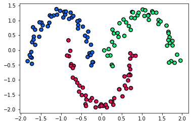
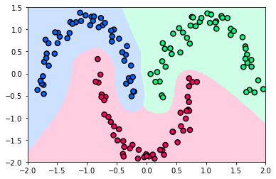
The next figure shows a toy dataset of \(N_{\rm samples}=150\) vectors in a space of \(N_{\rm input}=2\) dimensions divided in \(N_{\rm output}=3\) classes. Here, the points \({\rm x}_n\) colored blue have the label \(c_n=1\), those colored red have the label \(c_n=2\), and those colored green have the label \(c_n=3\).

Layer

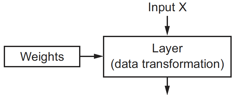
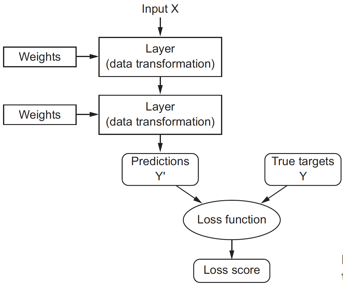
The building block of a neural network is the layer, which can be thought of as a filter for the data. Some layers are stateless, but more frequently layers have a state represented by a bunch of numbers called parameters or weights. The transformation implemented by a stateful layer is parameterized by its weights.

Neural network

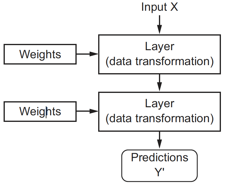
Neural networks consist of layers clipped together to implement a form of progressive data distillation. The most common network is a linear stack of layers, mapping a single input vector to a single output vector. But even so, there are two key architecture decisions to be made: how many layers to use, and how many hidden units to chose for each layer. These choices control “how much freedom” you are allowing the network to have when learning internal representations. Picking the right network architecture is more an art than a science. Although there are some best practices and principles you can rely on, only practice can help you become a proper neural network architect.

Cost function

Initially, the parameters of all layers are randomly initialized, so the network merely implements a series of random transformations. To control the output of a neural network, we need to be able to measure how far this output is from what you expected. This is the job of the loss function: it takes the network output and the true target (what you wanted the network to output) and computes a score expressing how bad the network has done on this specific example.

Choosing the right loss function for the right problem is extremely important, as a network will take any shortcut it can to minimize the loss. So, if the loss doesn’t fully correlate with success for the task at hand, our network will end up doing things you may not have wanted. Fortunately, when it comes to common problems such as classification and regression, there are simple guidelines we can follow to choose the correct loss:

• Cross entropy for classification problems,

• Mean squared error for regression problems.

Training

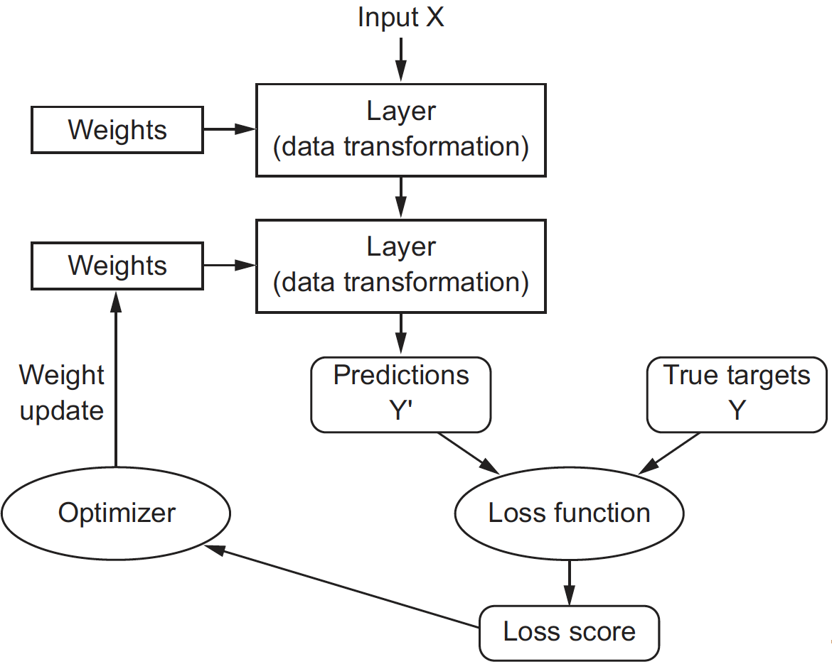
Training a neural network consists of using the loss function as a feedback signal to adjust the layer parameters such that the network will correctly map the inputs to their expected targets. Let’s discuss in more details how this happens concretely.

• You are given a set of input-output vectors describing a classification task. The output vectors are one-hot encoded.

\[ \mathcal{S} = \big\{ ({\rm x}_n,{\rm y}_n) \in\mathbb{R}^{N_{\rm input}}\times\mathbb{R}^{N_{\rm output}} \;|\; n=1,\dots,N_{\rm samples} \big\} \]

• You have also defined a two-layer neural network. This is a function from \(\mathbb{R}^{N_{\rm input}}\) to \(\mathbb{R}^{N_{\rm output}}\), whose computation is controlled by the layer parameters \(\theta=(W^{[1]},{\rm b}^{[1]},W^{[2]},{\rm b}^{[2]})\) according to the formula

\[ f_\theta({\rm x}) = {\sf softmax}\big({\sf relu}\big({\rm x}^\top W^{[1]} + {\rm b}^{[1]}\big) W^{[2]} + {\rm b}^{[2]}\big). \]

• Your goal is to adjust the layer parameters \(\theta\) such that the network output \(f_\theta({\rm x}_n)\) is close to the expected output \({\rm y}_n\) for every training example \(({\rm x}_n, {\rm y}_n)\). The cross entropy does a great job in measuring “how bad” the network has done on each specific example. Consequently, you want to

\[ \operatorname*{minimize}_{\theta} \underbrace{\sum_{n=1}^{N_{\rm samples}} \!\!-{\rm y}_n^\top \log\big(f_\theta({\rm x}_n)\big)}_{J(\theta)}. \]

• What comes next is to gradually adjust the network parameters, based on the training data. To this end, you can take advantage of the fact that all operations used in the network are differentiable, and compute the gradient of the cross entropy with regard to the network parameters. You can then move the parameters in the opposite direction from the gradient to decrease the cross entropy, which boils down to $\( \begin{aligned} \\ \theta_{k+1} = \theta_k - \alpha \nabla J(\theta_k).\\ \\ \end{aligned} \)$ This gradual adjustment is basically the training that deep learning is all about. You will eventually end up with a network that has a very low cross-entropy on its training data. The network has “learned” to map its inputs to outputs that are as close as they can be to the correct targets.

Prediction

After having trained a network, you will want to use it to make predictions. Remember that the network generates a vector of probabilities, each indicating how likely it is that the input belongs to one of the classes. Therefore, for a given input, the most probable class can be obtained as the maximum argument of the probabilities returned by the network.

\[ \textrm{prediction}({\rm x}) = \arg\max f_\theta({\rm x}) \]

In the moon dataset, the inputs are vectors of \(\mathbb{R}^2\). A nice experiment for testing the capabilities of your trained network is to sample the \(\mathbb{R}^2\) space over a fine grid, and predict the class of each point. The next figure shows the results of this experiment, where the sampled points are colored according to predicted class: blue for class 1, red for class 2, and green for class 3. You can see that the the network learned to correctly classify the training points.

It is also interesting to analyze the boundaries between the colored regions. If you train a network with a different architecture, you will see different region boundaries. Small networks will lead to straighter lines, whereas big networks will result in more bent curves. This is not surprising, as the number and the size of layers in a network affect its capacity to learn complex patterns from the training data.

Stochastic gradient descent

Having a good optimization algorithm can be the difference between waiting days versus just a few hours to get a good result. In this regard, “stochastic” gradient descent is a variant of the gradient method that can speed up learning, and perhaps even get you to a better final value for the cost function. What change is that you would be computing gradients on just few training examples at a time, rather than on the whole training set. This requires two ingredients.

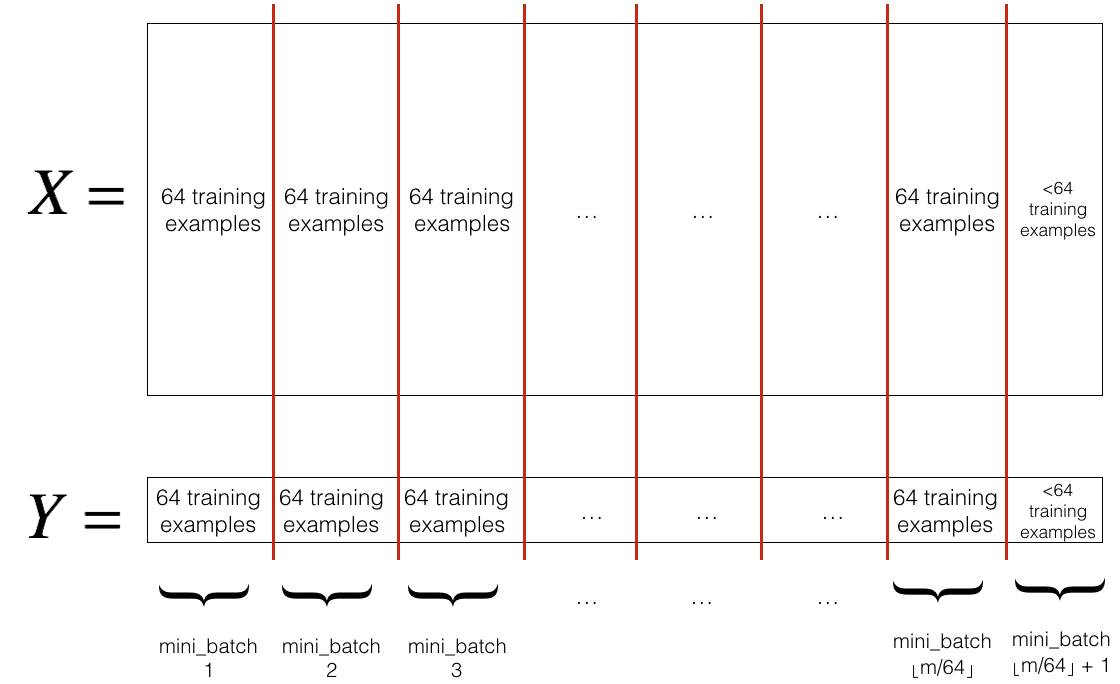
• Shuffling: Create a shuffled version of the training set \(X, Y\) by randomly permuting their rows. This random shuffling is done synchronously between \(X\) and \(Y\), so that after the shuffling the \(n^{th}\) row of \(X\) is the example corresponding to the \(n^{th}\) label in \(Y\). Shuffling ensures that examples will be split randomly into different mini-batches.

• Partition: Divide the shuffled \(X, Y\) into small batches of rows, as shown below (matrices are transposed for visualization purposes). Note that the number of training examples is not always divisible by the batch size, in which case the last batch might be smaller.

Closing remarks - Autograd vs TensorFlow vs PyTorch

In this assignment, you will solve the optimization problem that arises when training a neural network. You will use Autograd to do this, which provides a set of techniques to numerically evaluate the derivative of a function written in Python. Automatic differentiation exploits the fact that every computer program, no matter how complicated, executes a sequence of elementary operations. By applying the chain rule repeatedly to these operations, derivatives of arbitrary order can be computed automatically. Note however that automatic differentiation is neither symbolic nor numerical differentiation!

While Autograd is great for taking your first steps with automatic differentiation, there exist more advanced packages that you should be aware of, especially if you wish to start a career in data science.

• TensorFlow is mostly used in production by professional machine learning developers, software architects, and company programmers.

• PyTorch is more popular among researchers, data analysts, and Python developers.

Nowadays, both packages offer the same functionalities. There are no compelling reasons to prefer one over the other, apart from a matter of personal preference. They are both perfectly fine for more ambitious machine learning projects. Just pick one and start learning already!

Acknowledgment

Part of this chapter is based on the textbook Deep Learning with Python (1st ed., 2017) written by François Chollet.