5.6. Alternating gradient descent

There exists a modified version of projected gradient descent, in which only a subset of variables is updated at each step of the optimization process. This approach is based on the idea that the minimization of a differentiable function can be achieved by minimizing with respect to one variable at a time. However, an additional condition is required in the context of constrained optimization. The feasible set \(\mathcal{C}\subset \mathbb{R}^N\) must be “separable”, meaning that it can be decomposed as the cartesian product of two subsets \(\mathcal{C}_x\subset \mathbb{R}^{N_x}\) and \(\mathcal{C}_y \subset \mathbb{R}^{N_y}\) with \(N=N_x+N_y\). Put another way, alternating minimization requires that a constrained optimization problem is formulated as

\[\begin{split} \operatorname*{minimize}_{{\bf x},\, {\bf y}} % ({\bf x},\, {\bf y})\in\mathbb{R}^{N_x}\times\mathbb{R}^{N_y} \quad J({\bf x}, {\bf y}) \quad\textrm{subject to}\quad \begin{cases} {\bf x}\in\mathcal{C}_x \\ {\bf y}\in\mathcal{C}_y. \end{cases} \end{split}\]

Note that the constraint \(({\bf x}, {\bf y}) \in \mathcal{C}_x\times\mathcal{C}_y\) is less general than the constraint \(({\bf x}, {\bf y}) \in \mathcal{C}\). Nonetheless, such narrower class of problems can often be more efficiently solved through alternating gradient descent, which is guaranteed to work correctly under the assumption that

• the function \(J({\bf x}, {\bf y})\) is Lipschitz differentiable,

• the feasible sets \(\mathcal{C}_x\) and \(\mathcal{C}_y\) are convex (or the overall criterion satisfies the Kurdyka-Lojasiewicz property).

Keep in mind however that this algorithm does not work in general if the cost function is not continuously differentiable.

5.6.1. Algorithm

The necessary optimality condition states that if the point \((\bar{\bf x}, \bar{\bf y})\) is a minimum of \(J({\bf x}, {\bf y})\) on the feasible set \(\mathcal{C}\), then the negative gradient is “orthogonal” to \(\mathcal{C}\) there. When the feasible set is convex and separable, such condition can be equivalently expressed through the partial gradients \(\nabla_x J({\bf x}, {\bf y})\) and \(\nabla_y J({\bf x}, {\bf y})\). This yields the following implication, which becomes an equivalence when \(J({\bf w})\) is convex:

\[\begin{split} (\bar{\bf x}, \bar{\bf y}) \in \operatorname*{Argmin}_{({\bf x}, {\bf y})\in\mathcal{C}_x\times\mathcal{C}_y}\; J({\bf x}, {\bf y}) \qquad\implies\qquad \begin{cases} \bar{\bf x} = \mathcal{P}_{\mathcal{C}_x}\big(\bar{\bf x}-\alpha_x \nabla_x J(\bar{\bf x}, \bar{\bf y})\big) \\[1em] \bar{\bf y} = \mathcal{P}_{\mathcal{C}_y}\big(\bar{\bf y}-\alpha_y \nabla_y J(\bar{\bf x}, \bar{\bf y})\big). \end{cases} \end{split}\]

The above optimality condition motivates an efficient algorithm for constrained optimization. Given an initial point \((\bar{\bf x}_0, \bar{\bf y}_0)\) as well as two step-sizes \(\alpha_x>0\) and \(\alpha_y>0\), the optimization process consists of alternating a projected gradient step on the variable \({\bf x}\), and a projected gradient step on the variable \({\bf y}\), always using the most up-to-date iterates.

Alternating gradient descent

\[\begin{split} \left\lfloor \begin{aligned} {\bf x}_{k+1} &= \mathcal{P}_{\mathcal{C}_x}\big({\bf x}_k - \alpha_x \nabla_x J({\bf x}_k, {\bf y}_k)\big) \\[1em] {\bf y}_{k+1} &= \mathcal{P}_{\mathcal{C}_y}\big({\bf y}_k - \alpha_y \nabla_y J({\bf x}_{k+1}, {\bf y}_k)\big) \end{aligned} \right. \end{split}\]

This alternating scheme is illustrated in the figure below for a convex function of two variables \((x,y)\) subject to non-negativity constraints \(x\ge0\) and \(y\ge0\), so that the feasible set is separable. Moving the slider from left to right animates each step of alternating gradient descent. The white dots mark the sequence of iterates \((x_0, y_0), (x_1, y_1), \dots, (x_k, y_k)\) generated by the algorithm. The dashed lines show the trajectory travelled by a projected gradient step on the variable \(x\) (while the other is fixed), followed by a projected gradient step on the variable \(y\) (while the other is fixed). Note the ability of the algorithm to stop at the constrained minimum.

5.6.1.1. Step size

The alternating gradient method comes equipped with two step-sizes to control the distance travelled at each step. When the function is Lipschitz-differentiable, the curvature of the function is bounded with respect to each variable while fixing the other. It is then possible to define two constants \(L_x({\bf y})\) and \(L_y({\bf x})\) as follows

\[\begin{split} \begin{aligned} (\forall {\bf x}', {\bf x}''\in\mathbb{R}^{N_x}) &\qquad \big\|\nabla J({\bf x}', {\bf y}) - \nabla J({\bf x}'', {\bf y}) \big\| \le L_x({\bf y}) \, \big\|{\bf x}' - {\bf x}'' \big\| \\[1em] (\forall {\bf y}', {\bf y}''\in\mathbb{R}^{N_y}) &\qquad \big\|\nabla J({\bf x}, {\bf y}') - \nabla J({\bf x}, {\bf y}'') \big\| \le L_y({\bf x}) \, \big\|{\bf y}' - {\bf y}'' \big\|. \end{aligned} \end{split}\]

Alternating gradient descent is guaranteed to converge for any sequence of step-sizes such that

\[ (\forall k\in\mathbb{N})\qquad \alpha_{x}^{(k)} < \frac{1}{L_x({\bf y}_k)}, \qquad \alpha_{y}^{(k)} < \frac{1}{L_y({\bf x}_{k+1})}. \]

However, this may be a conservative choice, and the preferred approach is to determine a sufficiently small pair of step-sizes through a trial-and-error strategy guided by the analysis of the convergence plot.

5.6.1.2. Numerical implementation

Here is the python implementation of alternating gradient descent.

def alternating_gradient_descent(cost_fun, init, alpha, epochs, project=(lambda x: x, lambda y: y)):
    """
    Finds the minimum of a differentiable function subject to block-separable constraints.
    
    Arguments:
    cost_fun -- cost function | callable that takes '(x,y)' and returns 'J(x,y)'
    init     -- initial point | tuple of vectors
    alpha    -- step-sizes    | tuple of positive numbers
    epochs   -- n. iterations | integer
    project  -- projections   | tuple of callables, each takes 'u' and returns 'P(u)'
    
    Returns:
    (x,y)   -- minimum point | tuple of vectors
    history -- cost values   | list of scalars
    """
    import numbers
    if callable(project): project = project, project
    if isinstance(alpha, numbers.Number): alpha = alpha, alpha
        
    # Automatic gradient
    from autograd import grad 
    x_partial_grad = grad(cost_fun, 0)
    y_partial_grad = grad(cost_fun, 1)

    # Initialization
    x = np.array(init[0], dtype=float)
    y = np.array(init[1], dtype=float)

    # Iterative refinement
    history = []
    for k in range(epochs):
        
        # Projected gradient step
        x = project[0](x - alpha[0] * x_partial_grad(x,y))
        y = project[1](y - alpha[1] * y_partial_grad(x,y))
        
        # Bookkeeping
        history.append(cost_fun(x,y))
        
    return (x,y), history

5.6.2. Motivation

The standard projected gradient descent is guaranteed to converge with a sufficiently small step-size. Ideally, the step-size should be approximately the reciprocal of the maximum curvature of the function being minimized. The trouble arises when the curvature is highly variable in different directions, so that it is difficult to choose a step-size that guarantees good convergence in all dimensions. This could happen for quadratic or non-quadratic functions with elliptical geometry, particularly when their second derivatives are unbounded (the gradient is not Lipschitz-continuous). In these cases, one sets a small step-size according to an upper bound on the global curvature across dimensions (Lipschitz constant of the gradient). It is often harmful to increase the step-size, because doing so might lead the algorithm to diverge along some dimensions, or in some parts of the search space. At the same time, such a small step-size is highly conservative in other parts of the search space, leading to a very slow convergence. This is the sort of situation where alternating gradient descent helps.

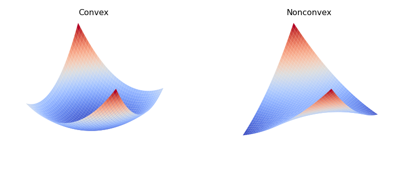
To illustrate the point, consider a simple quadratic function of two variables

\[\begin{split} J(x, y) = \begin{bmatrix}x\\y\end{bmatrix}^\top \underbrace{\begin{bmatrix}1 & a\\ a & 1\end{bmatrix}}_{A} \begin{bmatrix}x\\y\end{bmatrix} = x^2 + y^2 + 2axy. \end{split}\]

Note that the matrix \(A\) is semi-positive definite when \(|a| \le 1\), meaning that the function \(J(x,y)\) is convex. The matrix \(A\) is indefinite when \(|a| > 1\), resulting in the function \(J(x,y)\) being nonconvex. Two examples are shown below.

Eigenvalues of a \(2\times2\) matrix

The eigenvalues of the matrix \(\begin{bmatrix}d_1 & b\\ c & d_2\end{bmatrix}\) are the solutions to \(\lambda^2 -(d_1+d_2)\lambda + (d_1 d_2 - bc) = 0\), that is

\[\lambda = \frac{(d_1+d_2) \pm \sqrt{(d_1+d_2)^2 - 4(d_1 d_2-bc)}}{2}.\]

Setting \(d_1 = d_2 = 2\) and \(b=c=2a\) leads to \(\lambda = 2(1 \pm |a|).\)

Regardless the value of \(a\), the function is Lipschitz differentiable with the maximum curvature given by

\[ L_\max = \sup_{x,y} \|\nabla^2 J(x,y)\|_2 = 2 \|A\|_2 = 2(|a|+1). \]

The maximum curvature with respect to each variable is instead equal to

\[ L_x = \sup_{x,y} \left|\frac{\partial^2 J(x,y)}{\partial x^2}\right| = 2, \qquad L_y = \sup_{x,y} \left|\frac{\partial^2 J(x,y)}{\partial y^2}\right| = 2. \qquad \]

When \(A\) is semi-positive definite (convex function), the difference between the global curvature \(L_\max\) and the coordinate-wise curvatures \(L_x\) or \(L_y\) is limited, because \(|a| \le 1\). When \(A\) is indefinite (nonconvex function), the constant \(|a|\) could be very large, resulting in a large difference between the global curvature \(L_\max\) and the coordinate-wise curvatures \(L_x\) or \(L_y\). Using alternating gradient descent to solve this problem allows the choice of two step-sizes \(\alpha_x = 1/L_x\) and \(\alpha_y=1/L_y\) that could be much larger than the step-size \(\alpha = 1/L_\max\) used in the standard (projected) gradient descent. This simple example motivates the use of alternating minimization to solve block-structured nonconvex problems.

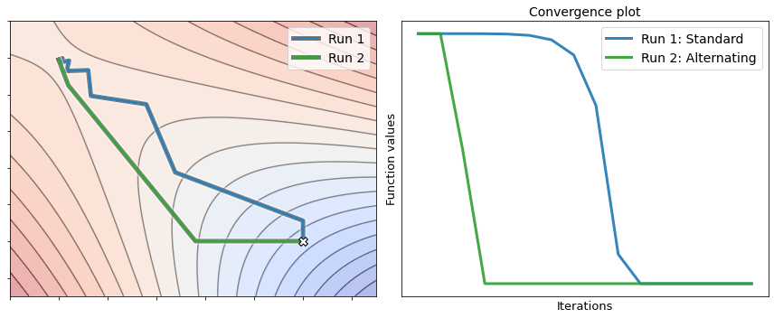
The figure below illustrates the resolution of the following problem

\[\begin{split} \operatorname*{minimize}_{(x,y)\in\mathbb{R}^2}\quad x^2 + y^2 + 2axy \quad\textrm{subject to}\quad \begin{cases} -1 \le x \le 1\\ -1 \le y \le 1. \end{cases} \end{split}\]

The choice \(a=2\) leads to a nonconvex problem with two optimal solutions: \((-1,1)\) and \((1,-1)\). The blue and the green lines trace the sequence of points generated by standard gradient descent (run 1) and alternating gradient descent (run 2), respectively. Remark that the latter converges in less iterations than the former. This confirms the insight that alternating gradient descent could be more effective than its standard counterpart in solving structured nonconvex problems.