Constant step-size#
Gradient descent works by moving along the negative gradient direction, thus generating the sequence
The step-size \(\alpha>0\) controls the distance travelled along the negative gradient direction at each iteration. More precisely, the distance between two consecutive iterates \({\bf w}_k\) and \({\bf w}_{k+1}\) is equal to the gradient magnitude scaled by the step-size:
If the step-size is chosen sufficiently small, the algorithm will stop near a stationary point of the function \(J({\bf w})\).
Trial and error#
Often in practice, the choice of step-size is done by trial and error. This consists of running gradient descent several times, using a different step-size on each attempt. The most common strategy is to use a fixed value for all the iterations, which usually takes the form of \(\alpha=10^{−m}\), with \(m\) being a positive integer. The general principle is illustrated in the next figure, which animates the first \(10\) iterations of gradient descent on a simple quadratic function. The left panel shows the points generated by gradient descent, whereas the right panel shows the convergence plot. Moving the slider runs gradient descent with a slightly different step-size. Here are some important considerations that are true in general.
When the step-size is too small, gradient descent moves slowly and requires more iterations to converge.
When the step-size is neither too small nor too large, gradient descent converges as fast as possible.
When the step-size is too large, gradient descent oscillates and needs more iterations to converge.
When the step-size is way too large, gradient descent diverges from the minimum.
Note that the notions of “small” and “large” are relative, and depend completely on the specific function being minimized.
Number of iterations#
How many iterations are needed by gradient descent to reach a minimum? Unfortunately, there is no precise answer to this question. The common practice is to stop gradient descent after a fixed number of iterations. While not being rigorous, this approach is practical and fast. Keep in mind however that the number of iterations required to converge is affected by the step-size. Smaller step-sizes require many iterations to achieve a significant progress. Larger step-sizes instead require less iterations, but at the risk that gradient descent bounces around erratically and never localizes an adequate solution. Consequently, the combination of step-size and number of iterations are best chosen together.
This concept is illustrated in the animation below, where the goal is to minimize the Rosenbrock function with gradient descent. By looking at the contour lines plotted in the background, you can notice that the (unique) minimum of this function is inside a long, narrow, parabolic shaped flat valley. Finding the valley is trivial, but converging to the minimum is challenging, because the gradient is highly variable inside the valley. The only way to guarantee the convergence is to choose a very small step-size. It is indeed harmful to increase the step-size beyond a certain threshold, because doing so leads the algorithm to diverge as soon as it reaches the narrow part of the valley. However, a small step-size requires a large number of iterations, otherwise the algorithm will not reach the minimum. Move the sliders below to find a good balance between these two parameters. The sequence of points generated by gradient descent is plotted in orange. You can also click and drag the circle with the little hand to move the initialization.
Oscillations are not always bad#
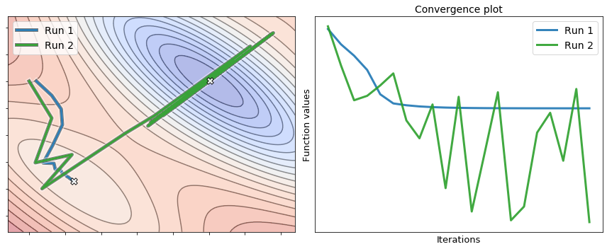
Since the cost functions are generally far too high dimensional to be visualized, the convergence plot is the only available feedback to guide the selection of a proper step-size. When doing so, it is not ultimately important that the convergence plot be strictly decreasing, i.e., that the function value decreases at every iteration. What matters is to find a step-size such that gradient descent converges as quickly as possible to the lowest possible value of the function. In other words, the best choice of step-size for a given optimization problem might be the one causing gradient descent to “hop around” a little bit, rather than the one ensuring a steady descent at each and every iteration.
The next figure shows two runs of gradient descent to minimize a nonconvex function. The first run uses a small step-size, whereas the second run uses a large step-size. It is interesting to analyze their behavior by looking at the convergence plot. The first run (small step-size) achieves a descent at each iteration, but it merely converges to a local minimum. Conversely, the second run (large step-size) oscillates wildly and never comes to a stop, but it escapes the local minimum and reaches the valley where the global minimum is located. While the second run does not converge, a simple fix is to slowly diminish the step-size during the optimization process, so as to damp and eventually remove the oscillations hindering the convergence. This is called step-size scheduling and will be covered in another section.