5.7.4. Example 9#
Collaborative filtering is a technique used by recommender systems to predict the rating a user would give to an item. The underlying assumption is that if a person A has the same opinion as a person B on an issue, A is more likely to have B’s opinion on a different issue than that of a randomly chosen person. Typically, the workflow of a collaborative filtering system includes two steps: one user expresses his preferences by rating items, and the system looks for people who share the same rating patterns to create suggestions. There are many ways to decide which users are similar and combine their choices to create a list of recommendations. This section will explain the approach based on non-negative matrix factorization.
5.7.4.1. Matrix factorization#
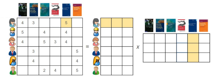
Recommendation algorithms need data about a set of items and a set of users who rated them. These ratings are organized in the form of a user-item matrix, where each row contains the ratings given by a user, and each column contains the ratings received by an item. The user-item matrix is very sparsely populated, since one user has likely rated only a small portion of the items available. Hence, dimensionality reduction is a possible way for recommendation algorithms to intelligently guess the values of every missing entry in such matrix. There are various methods to do this. Matrix factorization can be seen as breaking down a large matrix into a product of two smaller matrices having a common dimension. The reduced matrices actually represent the users and items individually. The rows in the first matrix represent the users, whereas the columns in the second matrix represent the items. Here is an example of how matrix factorization looks like.
5.7.4.1.1. Notation#
In what follows, the letter \(N\) indicates the number of users, and the letter \(M\) indicates the number of items. The (partial) ratings given by the users are gathered into a \(N\times M\) matrix.
Matrix factorization relies on the assumption that the matrix \({\bf Z}\in\mathbb{R}^{N \times M}\) can be approximately reduced to the product of two matrices \({\bf X}\in\mathbb{R}^{N \times K}\) and \({\bf Y}\in\mathbb{R}^{K \times N}\) having a common dimension \(K\). The rows in the matrix \({\bf X}\) represent the users, and the columns of the matrix \({\bf Y}\) represent the items.
Since the users only rated a small portion of the items available, the known ratings are indicated by the set of indices
5.7.4.1.2. Example#
Before going any further, it is helpful to make the problem more concrete. Let’s consider the purchases in a grocery store. The following is a simple example of user-item matrix. As you can see below, only few purchases are available for each client.
| Vegetables | Fruits | Sweets | Bread | Coffee | |
|---|---|---|---|---|---|
| John | 2 | 1 | |||
| Alice | 1 | 3 | 1 | 2 | |
| Mary | 1 | 1 | 3 | ||
| Greg | 1 | 1 | 4 | ||
| Peter | 2 | 2 | 1 | 1 | 1 |
| Karen | 2 | 2 | 1 | 1 |
The matrix itself is stored in the variable Z, and the indices of available purchases are stored in the variable idx.
Z = np.array([[0, 2, 1, 0, 0],
              [1, 3, 1, 2, 0],
              [0, 1, 1, 3, 0],
              [1, 1, 0, 4, 0],
              [2, 2, 1, 1, 1],
              [2, 2, 1, 1, 0]])

idx = Z.nonzero()
5.7.4.2. Optimization problem#
Matrix factorization is the problem of finding two small matrices \({\bf X}\) and \({\bf Y}\) that approximately reconstruct a larger matrix \({\bf Z}\) when multiplied. Specifically, the rating given by the user \(i\) to the item \(j\) must be reconstructed as the scalar product between the row \({\bf x}_i\) representing the user \(i\) and the column \({\bf y}_j\) associated to the item \(j\), so leading to the approximation
which can be rendered in matrix form as
This task can be equivalently formulated as the minimization of the square error between the known ratings and their reconstructions. It is additionaly required that all three matrices have non-negative elements for easier interpretation. Such considerations lead to the constrained optimization problem formulated as follows:
While the above problem only considers the known ratings indicated by the set \(\mathcal{I}\), the optimal matrices \(\bar{\bf X}\) and \(\bar{\bf Y}\) are defined for every user and every item. Hence, the product \(\bar{\bf Z} = \bar{\bf X}\bar{\bf Y}\) will give all the ratings, including the missing ones.
5.7.4.2.1. Feasible set#
In this example, the feasible set is the non-negative orthant, defined as
The projection onto the non-negative orthant consists of zeroing the negative elements and leaving the others untouched
More details can be found in the section discussing the projection onto a box.
5.7.4.3. Numerical resolution#
The optimization problem can be numerically solved with projected gradient descent in three steps:
implement the cost function with NumPy operations supported by Autograd,
implement the projection onto the feasible set,
select the initial point, the step-size, and the number of iterations.
5.7.4.3.1. Cost function#
Let’s start with the cost function. The implementation consists of a Python function that takes two arguments X and Y representing the matrices \({\bf X}\) and \({\bf Y}\) in the formula. Note that it is easier to compute all the errors, and then select the entries related to the available ratings with numpy’s advanced indexing.
def cost_fun(X, Y):
    error = Z - X @ Y
    return np.mean(error[idx]**2)
5.7.4.3.2. Initialization#
Let’s move to the initialization. The factors \({\bf X}\) and \({\bf Y}\) are created using the dimensions \(N\) and \(M\) of the rating matrix \({\bf Z}\). The common dimension \(K\) is arbitrarily chosen.
np.random.seed(42)

n, m = Z.shape

k = 3
X = np.random.rand(n, k)
Y = np.random.rand(k, m)
5.7.4.3.3. Flattening#
Now a technicality is needed. The standard implementation of gradient descent assumes that the cost function takes one input. But the cost function implemented earlier takes two inputs. To circumvent this issue, the freshly initialized matrices X and Y must be reshaped and concatenated into a single vector. Autograd provides the function flatten to do exactly this. In the code below, it takes the matrices X and Y packed in a tuple, and returns a vector flat_init that concatenates all the elements in X and Y. It also returns the function unflatten that reverts a vector back into the original matrices. Then, the conflict is solved by defining a new function flat_cost_fun that takes a vector w, transforms it into a tuple (X, Y) with the function unflatten, unpacks the matrices X and Y via the * syntax, and passes them to the cost function implemented earlier. The “flatten” cost function is what will be used for gradient descent.
from autograd.misc.flatten import flatten

flat_init, unflatten = flatten((X,Y))

flat_cost_fun = lambda w: cost_fun(*unflatten(w))
5.7.4.3.4. Projection#
Let’s proceed with the implementation of the projection. Since the cost function has been flattened, internally gradient descent will work with a single vector containing all the variables to be optimized. The projection is thus implemented by a Python function that takes just a single input. The cell below implements the projection onto the nonnegative orthant.
project_noneg = lambda w: np.maximum(0, w)
5.7.4.3.5. Execution#
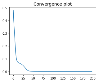
Now it remains to set the step-size, the number of iterations, and then run projected gradient descent. Note that the “flatten” cost function and the “flatten” initialization are used. This implies that the solution returned by the algorithm is also “flatten”, and it must be unflattened to retrieve the optimal matrices \(\bar{\bf X}\) and \(\bar{\bf Y}\).
alpha = 1
epochs = 200

w, history = gradient_descent(flat_cost_fun, flat_init, alpha, epochs, project_noneg)

Xopt, Yopt = unflatten(w)
The optimal matrices \(\bar{\bf X}\) and \(\bar{\bf Y}\) are shown in the following.
| 0 | 1 | 2 | |
|---|---|---|---|
| John | 0.72 | 0.90 | 0.44 |
| Alice | 1.70 | 0.12 | 0.43 |
| Mary | 0.06 | 0.94 | 1.27 |
| Greg | 0.42 | 0.14 | 1.80 |
| Peter | 0.62 | 1.14 | 0.08 |
| Karen | 0.62 | 1.14 | 0.08 |
| Vegetables | Fruits | Sweets | Bread | Coffee | |
|---|---|---|---|---|---|
| 0 | 0.39 | 1.68 | 0.46 | 0.63 | 0.51 |
| 1 | 1.52 | 0.83 | 0.60 | 0.38 | 0.59 |
| 2 | 0.34 | 0.10 | 0.32 | 2.04 | 0.12 |
Below are displayed the purchases reconstructed via the product \(\bar{\bf X}\bar{\bf Y}\). The values in the non-zero positions \((i,j)\in\mathcal{I}\) are equal to the original purchases \(z_{i,j}\), and the missing values have been guessed accordingly.
| Vegetables | Fruits | Sweets | Bread | Coffee | |
|---|---|---|---|---|---|
| John | 1.79 | 2.00 | 1.01 | 1.69 | 0.95 |
| Alice | 1.00 | 3.00 | 1.00 | 2.00 | 0.99 |
| Mary | 1.88 | 1.00 | 1.00 | 3.00 | 0.74 |
| Greg | 1.00 | 1.00 | 0.86 | 4.00 | 0.52 |
| Peter | 2.00 | 2.00 | 1.00 | 1.00 | 1.00 |
| Karen | 2.00 | 2.00 | 1.00 | 1.00 | 1.00 |
5.7.4.3.6. Alternating gradient descent#
Note that the feasible set is separable with respect to the matrices \({\bf X}\) and \({\bf Y}\). Hence, alternating minimization can be used. The implementation of alternating gradient descent assumes that the cost function takes two inputs. This is a happy coincidence, as the function cost_fun implemeted earlier also takes two inputs, and it can be passed directly to the algorithm without any “flattening” trickery. The initialization is a tuple packed with the matrices X and Y. The solution returned by the algorithm is also a tuple with the optimal matrices \(\bar{\bf X}\) and \(\bar{\bf Y}\).
init = X, Y
alpha = 2
epochs = 200

(Xalt, Yalt), histalt = alternating_gradient_descent(cost_fun, init, alpha, epochs, project_noneg)
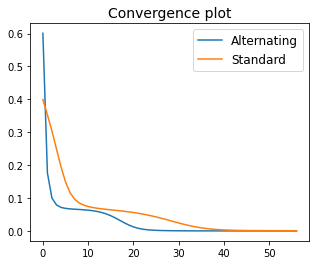
The advantage of alternating gradient descent is that it could work with a larger step-size. In this specific example, it converges with \(\alpha=2\), whereas standard gradient descent only converges with \(\alpha=1\). This means that alternaning gradient descent reaches a solution faster (i.e., in less iterations), as indicated by the convergence plots shown below.
Below are displayed the purchases reconstructed via the product \(\bar{\bf X}\bar{\bf Y}\). The solution found by alternating gradient descent is different than the one found by standard gradient descent. This occurs because the cost function is nonconvex and the optimal solution is not unique, namely the ratings matrix can be filled in different ways (all equivalent). Consequently, the two algorithms converge to different stationary points, because of the (slight) difference in their iterative updates.
| Vegetables | Fruits | Sweets | Bread | Coffee | |
|---|---|---|---|---|---|
| John | 0.86 | 2.00 | 1.00 | 2.18 | 0.86 |
| Alice | 1.00 | 3.00 | 1.00 | 2.00 | 1.19 |
| Mary | 0.12 | 1.00 | 1.00 | 3.00 | 0.44 |
| Greg | 1.00 | 1.00 | 1.61 | 4.00 | 0.62 |
| Peter | 2.00 | 2.00 | 1.00 | 1.00 | 1.00 |
| Karen | 2.00 | 2.00 | 1.00 | 1.00 | 1.00 |