5.4.10. Hypersphere

For a given scalar \(\xi \ge 0\), the hypersphere is a nonconvex constraint defined as

\[ \mathcal{C}_{\rm sphere} = \big\{ {\bf w} \in \mathbb{R}^{N} \;|\; \|{\bf w}\|_2 = \xi \big\}. \]

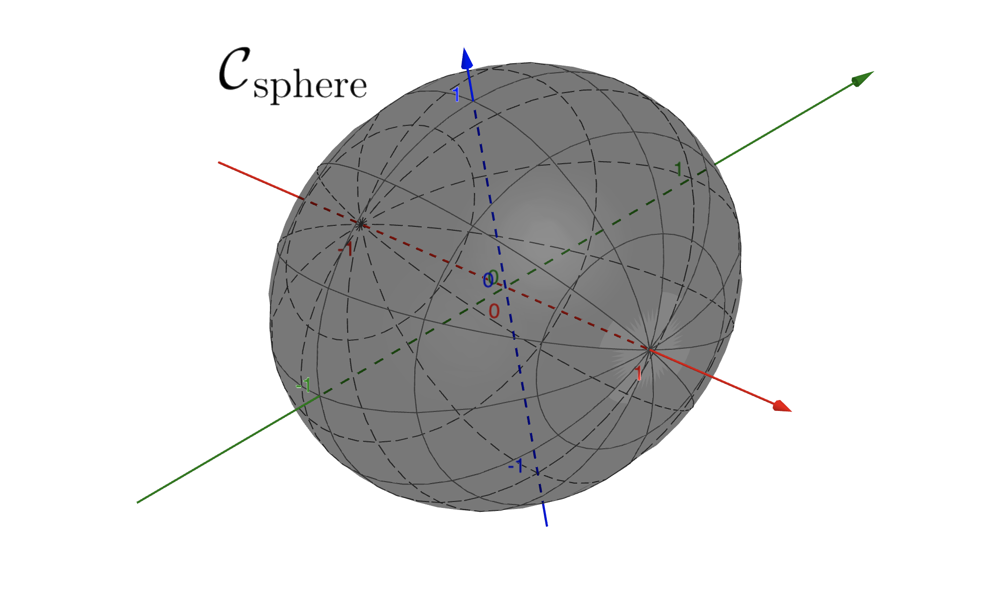
The condition \(\xi \ge 0\) allows this subset to be nonempty. The figure below shows how this constraint looks like in \(\mathbb{R}^{2}\) or in \(\mathbb{R}^{3}\).

Sphere in 2D

Sphere in 3D

5.4.10.1. Constrained optimization

Optimizing a function \(J({\bf w})\) subject to the hyphersphere constraint can be expressed as

\[ \operatorname*{minimize}_{\textbf{w}\in\mathbb{R}^N}\; J({\bf w}) \quad{\rm s.t.}\quad \|{\bf w}\|_2 = \xi. \]

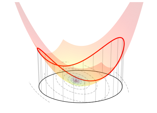
The figure below visualizes such an optimization problem in \(\mathbb{R}^{2}\).

5.4.10.2. Orthogonal projection

The projection of a point \({\bf u}\in\mathbb{R}^{N}\) onto the hypersphere is one of the possible solutions to the following problem

\[ \operatorname*{minimize}_{{\bf w}\in\mathbb{R}^N}\;\; \|{\bf w}-{\bf u}\|^2 \quad{\rm s.t.}\quad \|{\bf w}\|_2 = \xi. \]

The solution can be analytically computed as follows.

Projection onto the hypersphere

\[ \mathcal{P}_{\mathcal{C}_{\rm sphere}}({\bf u}) = {\bf u} \, \dfrac{\xi}{\|{\bf u}\|_2} \]

Note that the above expression is ill-defined when \({\bf u}={\bf 0}\). This stems from the fact that any point of the hypersphere is a valid projection of the zero vector. A possible convention is to set \(\mathcal{P}_{\mathcal{C}_{\rm sphere}}({\bf 0})=[\xi,0\dots,0]^\top\).

5.4.10.3. Implementation

The python implementation is given below.

def project_sphere(u, bound):
    
    assert bound >= 0, "The bound must be non-negative"
    
    if np.linalg.norm(u) < 1e-16:
        p = np.zeros(u.shape)
        p[0] = bound
    else:
        p = u * bound / np.linalg.norm(u)
        
    return p

Here is an example of use.

u = np.array([-1.2, 1.2])

p = project_sphere(u, bound=1)