4.6.3. Example 3#
Consider this optimization problem involving a nonconvex function of one variable defined as
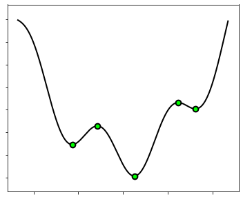
The cost function is shown below, where its stationary points are marked with a green dot.
4.6.3.1. Analytical approach#
Manually finding the global minimum of a nonconvex function is often a complicated matter. On the one hand, setting the first derivatives to zero yields a nonlinear equation that rarely provides closed-form solutions. On the other hand, the first derivatives vanishes not only in global minima, but also in local minima, global and local maxima, as well as saddle points. Moving the slider in the following figure plots the first derivative of the function. Take notice of the points where it passes through the zero: they are the stationary points of the function, among which there is the global minimum. Unfortunately, there is no way to know which is the global minimum by just looking at its derivative!
4.6.3.2. Numerical approach#
Numerical optimization is more difficult with nonconvex functions. The difficulty stems from the fact that gradient descent halts its progress in a stationary point, which is not guaranteed to be a global minimum, and sometimes not even a local minimum. Since gradient descent stops wherever the first derivative is equal to zero, a question naturally arises: which stationary point does gradient descent actually converge to? Clearly, it all depends on the initialization. The figure below shows several runs of gradient descent, each starting from a different initial point. Notice how each run ends up in a different minimum depending on where the initialization is located on the cost function.
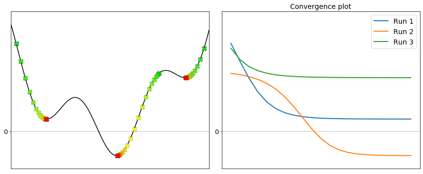
The best way to deal with nonconvexity is to run gradient descent with multiple initializations, and then compare the convergence plots. The solution corresponding to the lowest value attained on the cost function is probably the global minimum, or at least a better local minimum than the others. In the above example, the lowest value is attained by the second run, which happens to be the one that converged to the global minimum.
[Run 1] Final cost:  0.46421 ==> Solution found: -2.28413  (local  minimum)
[Run 2] Final cost: -0.92609 ==> Solution found:  0.53329  (global minimum)
[Run 3] Final cost:  2.03905 ==> Solution found:  3.26013  (local  minimum)
The take-away message is that the convergence plot is the primary tool to analyze the behavior of gradient descent.